PyVBMC Example 5: Prior distributions#
In this notebook, we discuss some considerations for using a prior distribution with PyVBMC, and demonstrate some convenient built-in priors.
This notebook is Part 5 of a series of notebooks in which we present various example usages for VBMC with the PyVBMC package. The code used in this example is available as a script here.
0. Preliminaries#
In Bayesian inference – and in PyVBMC – you need a prior over parameters, \(p(\theta)\). The prior should be a proper probability density function (pdf), i.e. a normalized distribution. A common choice is an independent or factorized prior:
where each prior \(p_{i}(\theta_{i})\) is chosen separately for each parameter \(\theta_{i}\). Note that an independent prior does not mean that the posterior is independent!
1. Specifying a prior with PyVBMC#
By default, as in the previous notebooks, PyVBMC assumes that the first argument to VBMC is a function which returns the log-joint (i.e., the sum of log-likelihood and log-prior). However, you may instead pass a function which returns the log-likelihood as a first argument, and supply the prior separately. Using the keyword log_prior, you may pass a function (of a single argument) which returns the log-density of the prior given a point:
vbmc = VBMC(log_likelihood, x0, lb, ub, plb, pub, log_prior=log_prior_function)
Alternatively, using the keyword prior, you may pass one of the following:
a PyVBMC prior imported from
pyvbmc.priorsthat matches the dimension of the model,an appropriate continuous
scipy.statsdistribution that matches the dimension of the model, ora list of univariate (i.e., one-dimensional) PyVBMC priors and/or continuous
scipy.statsdistributions, which are treated as independent priors for each parameter \(\theta_{i}\). In this case the length of the list should equal the dimension of the model.
vbmc = VBMC(log_likelihood, x0, lb, ub, plb, pub, prior=UniformBox(0, 1, D=2))
vbmc = VBMC(log_likelihood, x0, lb, ub, plb, pub, prior=scipy.stats.multivariate_normal(mu, cov))
vbmc = VBMC(log_likelihood, x0, lb, ub, plb, pub, prior=[UniformBox(0, 1), scipy.stats.norm()])
Below we detail the built-in PyVBMC priors (1) for various use-cases. See the relevant documentation for details on other types of priors, and the examples below for some usage cases.
import numpy as np
import scipy.stats as scs
from pyvbmc import VBMC
from pyvbmc.priors import UniformBox, Trapezoidal, SplineTrapezoidal, SmoothBox
import matplotlib.pyplot as plt

figsize = (8, 4)
2. Bounded parameters#
PyVBMC implements several priors for bounded parameters. All the priors listed below apply both to the univariate and to the multivariate case, with the assumption of independent/factorized priors mentioned above.
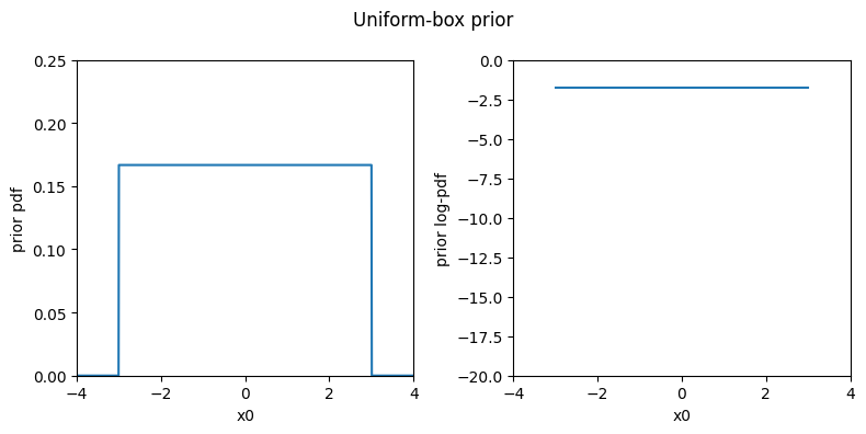
Uniform-box prior (UniformBox)#
For bounded parameters, the first simple choice is a non-informative uniformly flat prior between the hard bounds. This is implemented by the UniformBox multivariate prior. Below, we plot the pdf of the prior for a one-dimensional problem (the pdf to the left and the log-pdf to the right).
lb = -3
ub = 3
plb = -2
pub = 2
x = np.linspace(lb - 1, ub + 1, 1000)

prior = UniformBox(lb, ub)

fig, (ax1, ax2) = plt.subplots(1, 2, sharex=True, figsize=figsize)
ax1.plot(x, prior.pdf(x))
ax1.set_xlim(-4, 4)
ax1.set_ylim(0, 0.25)
ax1.set_xlabel("x0")
ax1.set_ylabel("prior pdf")
ax2.plot(x, prior.log_pdf(x))
ax2.set_ylim(-20, 0)
ax2.set_xlabel("x0")
ax2.set_ylabel("prior log-pdf")
plt.suptitle("Uniform-box prior")
fig.tight_layout()
# (Note that the log-pdf is not plotted where it takes values of -infinity.)
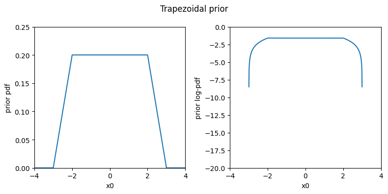
Trapezoidal prior (Trapezoidal)#
Alternatively, for each parameter we can define the prior to be flat within a range, where a reasonable choice is the “plausible” range, and then falls to zero towards the hard bounds. This is a trapezoidal or “tent” prior, implemented by the Trapezoidal prior shown below.
prior = Trapezoidal(lb, plb, pub, ub)

fig, (ax1, ax2) = plt.subplots(1, 2, sharex=True, figsize=figsize)
ax1.plot(x, prior.pdf(x))
ax1.set_xlim(-4, 4)
ax1.set_ylim(0, 0.25)
ax1.set_xlabel("x0")
ax1.set_ylabel("prior pdf")
ax2.plot(x, prior.log_pdf(x))
ax2.set_ylim(-20, 0)
ax2.set_xlabel("x0")
ax2.set_ylabel("prior log-pdf")
plt.suptitle("Trapezoidal prior")
fig.tight_layout()
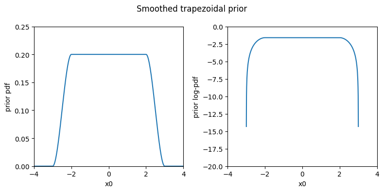
Spline-smoothed trapezoidal prior (SplineTrapezoidal)#
Finally, we can use a smoothed trapezoidal prior with soft transitions at the edges obtained using cubic splines. This prior is better behaved numerically as it is continuous with continuous derivatives (i.e., no sharp edges), so we recommend it over the simple trapezoidal prior. The spline-smoothed trapezoidal prior is implemented by the SplineTrapezoidal class.
prior = SplineTrapezoidal(lb, plb, pub, ub)

fig, (ax1, ax2) = plt.subplots(1, 2, sharex=True, figsize=figsize)
ax1.plot(x, prior.pdf(x))
ax1.set_xlim(-4, 4)
ax1.set_ylim(0, 0.25)
ax1.set_xlabel("x0")
ax1.set_ylabel("prior pdf")
ax2.plot(x, prior.log_pdf(x))
ax2.set_ylim(-20, 0)
ax2.set_xlabel("x0")
ax2.set_ylabel("prior log-pdf")
plt.suptitle("Smoothed trapezoidal prior")
fig.tight_layout()
3. Unbounded parameters#
If your variables are unbounded, remember that PyVBMC supports scipy.stats univariate and multivariate distributions, so you could use standard priors such as a multivariate normal distribution or a multivariate Student’s t distribution with 3-7 degrees of freedom.
See for example this page on the Stan wiki for a broader discussion on prior choice.
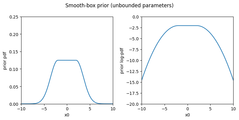
Smooth-box prior (SmoothBox)#
As an alternative to these common choices, we also provide a smooth-box distribution which is uniform within an interval (typically, the plausible range) and then falls with Gaussian tails with standard deviation(s) equal to scale outside the interval. The smoothbox prior is implemented by the SmoothBox class.
lb = -np.inf
ub = np.inf
plb = -2
pub = 2
# We recommend setting the scale as a fraction of the plausible range.
# For example `scale` set to 4/10 of the plausible range assigns ~50%
# (marginal) probability to the plateau of the distribution.
# Also similar fractions (e.g., half of the range) would be reasonable.
# Do not set `scale` too small with respect to the plausible range, as it
# might cause issues.
p_range = pub - plb
scale = 0.4 * p_range

prior = SmoothBox(plb, pub, scale)

x = np.linspace(plb - 2 * p_range, pub + 2 * p_range, 1000)
fig, (ax1, ax2) = plt.subplots(1, 2, sharex=True, figsize=figsize)
ax1.plot(x, prior.pdf(x))
ax1.set_xlim(x[0], x[-1])
ax1.set_ylim(0, 0.25)
ax1.set_xlabel("x0")
ax1.set_ylabel("prior pdf")
ax2.plot(x, prior.log_pdf(x))
ax2.set_ylim(-20, 0)
ax2.set_xlabel("x0")
ax2.set_ylabel("prior log-pdf")
plt.suptitle("Smooth-box prior (unbounded parameters)")
fig.tight_layout()
4. Using a prior with PyVBMC#
To conclude, we run inference on a couple of problems using some of the priors introduced in this notebook.
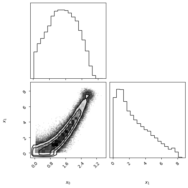
Bounded example#
In this example, we use the spline-smoothed trapezoidal prior (SplineTrapezoidal) introduced in this notebook. The code below shows several equivalent ways in which the prior can be set in PyVBMC (see the comments in the code below for details).
D = 2  # Still in 2-D
lb = np.zeros((1, D))
ub = 10 * np.ones((1, D))
plb = 0.1 * np.ones((1, D))
pub = 3 * np.ones((1, D))

# Define the prior and the log-likelihood
prior = SplineTrapezoidal(lb, plb, pub, ub)


def log_likelihood(theta):
    """D-dimensional Rosenbrock's banana function."""
    theta = np.atleast_2d(theta)

    x, y = theta[:, :-1], theta[:, 1:]
    return -np.sum((x**2 - y) ** 2 + (x - 1) ** 2 / 100, axis=1)


x0 = np.ones((1, D))
np.random.seed(42)
vbmc = VBMC(log_likelihood, x0, lb, ub, plb, pub, prior=prior)
# vbmc = VBMC(log_likelihood, x0, lb, ub, plb, pub, log_prior=prior.log_pdf)  # equivalently
# vbmc = VBMC(lambda x: log_likelihood(x) + prior.log_pdf(x), x0, lb, ub, plb, pub)  # equivalently
vp, results = vbmc.optimize()
vp.plot();
Beginning variational optimization assuming EXACT observations of the log-joint.
 Iteration  f-count    Mean[ELBO]    Std[ELBO]    sKL-iter[q]   K[q]  Convergence  Action
     0         10          -1.41         1.15    310361.34        2        inf     start warm-up
     1         15          -3.31         0.26        13.00        2        inf
     2         20          -3.05         0.02         0.36        2       9.32
     3         25          -3.03         0.01         0.20        2       4.89
     4         30          -3.02         0.00         0.04        2      0.947     end warm-up
     5         35          -3.06         0.00         0.01        2      0.332
     6         40          -3.02         0.00         0.00        2      0.193
     7         45          -2.71         0.00         0.07        5       2.74
     8         50          -2.64         0.00         0.05        6        1.4     rotoscale, undo rotoscale
     9         55          -2.59         0.01         0.01        7      0.536
    10         60          -2.55         0.00         0.00       10      0.203
    11         65          -2.51         0.00         0.00       13       0.19
    12         70          -2.44         0.00         0.01       16      0.588
    13         75          -2.44         0.00         0.00       18     0.0273
    14         80          -2.43         0.00         0.00       19     0.0392
    15         85          -2.43         0.00         0.00       20      0.024     stable
   inf         85          -2.42         0.00         0.00       50      0.024     finalize
Inference terminated: variational solution stable for options.tol_stable_count fcn evaluations.
Estimated ELBO: -2.424 +/-0.002.
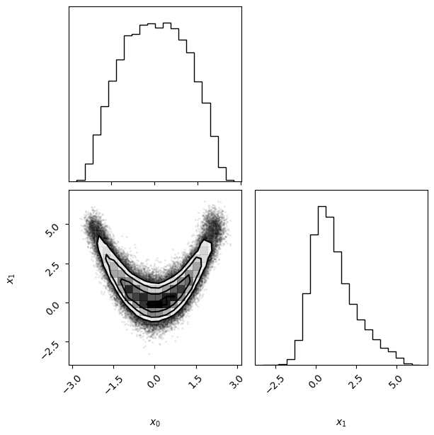
Unbounded example#
We run now another example with an unbounded prior. In this case, we apply a multivariate normal prior with zero mean and diagonal covariance, with variance \(\sigma^2 = 9\) in each dimension (we chose \(\sigma\) equal to half the plausible range).
Note that this is equivalent to setting a normal distribution separately for each variable. The code below shows a couple of equivalent ways in which the prior could be initialized in PyVBMC using scipy.stats distributions.
D = 2  # Still in 2-D
lb = np.full((1, D), -np.inf)
ub = np.full((1, D), np.inf)
plb = -3 * np.ones((1, D))
pub = 3 * np.ones((1, D))

# Define the prior as a multivariate normal (scipy.stats distribution)
scale = 0.5 * (pub - plb).flatten()
prior = scs.multivariate_normal(mean=np.zeros(D), cov=scale**2)
# prior = [scs.norm(scale=scale[0]),scs.norm(scale=scale[1])] # equivalently

x0 = np.zeros((1, D))
np.random.seed(42)
vbmc = VBMC(log_likelihood, x0, lb, ub, plb, pub, prior=prior)
vp, results = vbmc.optimize()
vp.plot();
Beginning variational optimization assuming EXACT observations of the log-joint.
 Iteration  f-count    Mean[ELBO]    Std[ELBO]    sKL-iter[q]   K[q]  Convergence  Action
     0         10          -3.17         0.83      5094.29        2        inf     start warm-up
     1         15          -2.90         0.08         0.24        2        inf
     2         20          -2.81         0.00         0.09        2       2.52
     3         25          -2.82         0.00         0.01        2       0.28
     4         30          -2.80         0.00         0.01        2      0.224     end warm-up
     5         35          -2.77         0.00         0.01        2      0.211
     6         40          -2.79         0.00         0.00        2      0.161
     7         45          -2.58         0.00         0.17        5       4.77
     8         50          -2.49         0.00         0.05        6       1.42
     9         55          -2.43         0.00         0.02        7      0.778     rotoscale, undo rotoscale
    10         60          -2.38         0.00         0.03       10       0.87
    11         65          -2.36         0.00         0.00       13      0.144
    12         70          -2.32         0.00         0.00       16      0.165
    13         75          -2.32         0.00         0.01       18      0.183
    14         80          -2.31         0.00         0.00       18     0.0557     stable
   inf         80          -2.28         0.00         0.00       50     0.0557     finalize
Inference terminated: variational solution stable for options.tol_stable_count fcn evaluations.
Estimated ELBO: -2.280 +/-0.001.
Acknowledgments#
Work on the PyVBMC package was funded by the Finnish Center for Artificial Intelligence FCAI.