PyVBMC Example 4: Multiple runs as validation#
Here we explore running PyVBMC multiple times in order to validate the results: if the final variational posteriors obtained from several different initial points are consistent, we can be more confident that the results are correct.
This notebook is Part 4 of a series of notebooks in which we present various example usages for VBMC with the PyVBMC package. The code used in this example is available as a script here.
import numpy as np
import scipy.stats as scs
from scipy.optimize import minimize
from pyvbmc import VBMC
import matplotlib.pyplot as plt
1. Model definition#
We use the same toy target function as in Example 1, a broad Rosenbrock’s banana function in \(D = 2\), with unbounded parameters:
D = 2  # We'll use a 2-D problem for a quicker demonstration
prior_mu = np.zeros(D)
prior_var = 3 * np.ones(D)


def log_prior(theta):
    """Multivariate normal prior on theta."""
    cov = np.diag(prior_var)
    return scs.multivariate_normal(prior_mu, cov).logpdf(theta)


# log-likelihood (Rosenbrock)
def log_likelihood(theta):
    """D-dimensional Rosenbrock's banana function."""
    theta = np.atleast_2d(theta)

    x, y = theta[:, :-1], theta[:, 1:]
    return -np.sum((x**2 - y) ** 2 + (x - 1) ** 2 / 100, axis=1)


# Full model:
def log_joint(theta, data=np.ones(D)):
    """log-density of the joint distribution."""
    return log_likelihood(theta) + log_prior(theta)


LB = np.full((1, D), -np.inf)  # Lower bounds
UB = np.full((1, D), np.inf)  # Upper bounds
PLB = np.full((1, D), prior_mu - np.sqrt(prior_var))  # Plausible lower bounds
PUB = np.full((1, D), prior_mu + np.sqrt(prior_var))  # Plausible upper bounds
options = {
    "max_fun_evals": 50 * D  # Slightly reduced from 50 * (D + 2), for speed
}
2. Validation#
For validation, we recommend running PyVBMC 3-4 times from different initial points:
np.random.seed(42)
n_runs = 3
vps, elbos, elbo_sds, success_flags, result_dicts = [], [], [], [], []
for i in range(n_runs):
    print(f"PyVBMC run {i} of {n_runs}")

    # Determine initial point x0:
    if i == 0:
        x0 = prior_mu  # First run, start from prior mean
    else:
        x0 = np.random.uniform(PLB, PUB)  # Other runs, randomize
    # Preliminary maximum a posteriori (MAP) estimation:
    x0 = minimize(
        lambda t: -log_joint(t),
        x0.ravel(),  # minimize expects 1-D input for initial point x0
        bounds=[(-np.inf, np.inf), (-np.inf, np.inf)],
    ).x

    # Run PyVBMC:
    vbmc = VBMC(
        log_joint,
        x0,
        LB,
        UB,
        PLB,
        PUB,
        options=options,
    )
    vp, results = vbmc.optimize()

    # Record the results:
    vps.append(vp)
    elbos.append(results["elbo"])
    elbo_sds.append(results["elbo_sd"])
    success_flags.append(results["success_flag"])
    result_dicts.append(results)
PyVBMC run 0 of 3
Reshaping x0 to row vector.
Beginning variational optimization assuming EXACT observations of the log-joint.
 Iteration  f-count    Mean[ELBO]    Std[ELBO]    sKL-iter[q]   K[q]  Convergence  Action
     0         10          -1.69         0.80     73438.00        2        inf     start warm-up
     1         15          -1.80         0.08         1.20        2        inf
     2         20          -1.82         0.00         0.03        2      0.889
     3         25          -1.81         0.00         0.00        2     0.0555
     4         30          -1.81         0.00         0.00        2     0.0611     end warm-up
     5         35          -1.80         0.00         0.00        2       0.06
     6         40          -1.81         0.00         0.00        2      0.127
     7         45          -1.61         0.00         0.09        5       2.92
     8         50          -1.58         0.00         0.02        6       0.52     rotoscale, undo rotoscale
     9         55          -1.57         0.00         0.00        9     0.0435
    10         60          -1.56         0.00         0.00       12     0.0439
    11         65          -1.54         0.00         0.00       15     0.0994
    12         70          -1.53         0.00         0.01       17      0.192     stable
   inf         70          -1.53         0.00         0.01       50      0.192     finalize
Inference terminated: variational solution stable for options.tol_stable_count fcn evaluations.
Estimated ELBO: -1.527 +/-0.001.
PyVBMC run 1 of 3
Reshaping x0 to row vector.
Beginning variational optimization assuming EXACT observations of the log-joint.
 Iteration  f-count    Mean[ELBO]    Std[ELBO]    sKL-iter[q]   K[q]  Convergence  Action
     0         10          -1.39         0.60    183360.39        2        inf     start warm-up
     1         15          -1.79         0.17         5.72        2        inf
     2         20          -1.83         0.00         0.01        2      0.356
     3         25          -1.79         0.00         0.01        2      0.474
     4         30          -1.83         0.00         0.00        2      0.127     end warm-up
     5         35          -1.81         0.00         0.00        2      0.118
     6         40          -1.81         0.00         0.00        2     0.0519
     7         45          -1.62         0.00         0.11        5       3.22
     8         50          -1.60         0.00         0.00        6      0.176
     9         55          -1.55         0.00         0.01        9       0.34     rotoscale, undo rotoscale
    10         60          -1.55         0.00         0.01       12      0.207
    11         65          -1.54         0.00         0.00       15     0.0598
    12         70          -1.55         0.00         0.00       17     0.0632     stable
   inf         70          -1.52         0.00         0.00       50     0.0632     finalize
Inference terminated: variational solution stable for options.tol_stable_count fcn evaluations.
Estimated ELBO: -1.525 +/-0.000.
PyVBMC run 2 of 3
Reshaping x0 to row vector.
Beginning variational optimization assuming EXACT observations of the log-joint.
 Iteration  f-count    Mean[ELBO]    Std[ELBO]    sKL-iter[q]   K[q]  Convergence  Action
     0         10          -2.19         0.92     19097.79        2        inf     start warm-up
     1         15          -1.93         0.10         0.03        2        inf
     2         20          -1.84         0.00         0.03        2        1.1
     3         25          -1.85         0.00         0.01        2      0.178
     4         30          -1.86         0.00         0.00        2      0.047     end warm-up
     5         35          -1.83         0.00         0.00        2      0.113
     6         40          -1.85         0.00         0.00        2     0.0818
     7         45          -1.78         0.00         0.01        5      0.429
     8         50          -1.62         0.00         0.09        8       2.56     rotoscale, undo rotoscale
     9         55          -1.58         0.00         0.01        9      0.432
    10         60          -1.57         0.00         0.00       12     0.0779
    11         65          -1.54         0.00         0.00       15      0.147
    12         70          -1.53         0.00         0.01       17      0.249
    13         75          -1.53         0.00         0.00       18     0.0368     stable
   inf         75          -1.53         0.00         0.00       50     0.0368     finalize
Inference terminated: variational solution stable for options.tol_stable_count fcn evaluations.
Estimated ELBO: -1.529 +/-0.000.
We now perform some diagnostic checks on the variational solution. First, we check that the ELBO’s from different runs are close to each other (i.e. with a difference much smaller than 1):
print(elbos)
[-1.5273433504679828, -1.5248830970271374, -1.5290414540115609]
Then, we check that the variational posteriors from distinct runs are similar. As a measure of similarity, we compute the Kullback-Leibler divergence between each pair:
kl_matrix = np.zeros((n_runs, n_runs))
for i in range(n_runs):
    for j in range(i, n_runs):
        # The `kldiv` method computes the divergence in both directions:
        kl_ij, kl_ji = vps[i].kl_div(vp2=vps[j])
        kl_matrix[i, j] = kl_ij
        kl_matrix[j, i] = kl_ji
Note that the KL divergence is asymmetric, so we have an asymmetric matrix:
print(kl_matrix)
[[-0.          0.0126071   0.00961694]
 [ 0.01044285 -0.          0.0136719 ]
 [ 0.01059469  0.01364032 -0.        ]]
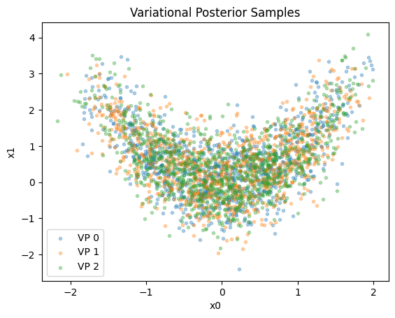
Ideally, we want all KL divergence matrix entries to be much smaller than 1. For a qualitative validation, we recommend a visual inspection of the posteriors:
for i, vp in enumerate(vps):
    samples, __ = vp.sample(1000)
    plt.scatter(
        samples[:, 0],
        samples[:, 1],
        alpha=1 / len(vps),
        marker=".",
        label=f"VP {i}",
    )
plt.title("""Variational Posterior Samples""")
plt.xlabel("x0")
plt.ylabel("x1")
plt.legend();
We can also check that convergence was acheived in all runs, according to PyVBMC (we want success_flag = True for each run):
print(success_flags)
[True, True, True]
Finally, we can pick the variational solution with highest ELCBO (the lower confidence bound on the ELBO).
beta_lcb = 3.0  # Standard confidence parameter (in standard deviations)
# beta_lcb = 5.0  # This is more conservative
elcbos = np.array(elbos) - beta_lcb * np.array(elbo_sds)
idx_best = np.argmax(elcbos)
print(idx_best)
1
The VariationalPosterior class implements save and load methods, similar to VBMC (as we saw in Example 3). We’ll save this best posterior to a file, so we can compare it against our results in Example 6:
vps[idx_best].save("noise_free_vp.pkl", overwrite=True)
3. Conclusions#
In this notebook, we have shown you some techniques to validate the results of PyVBMC by comparing statitics across multiple runs.
In the next notebook, we will demonstrate using PyVBMC with models in which the likelihood function is noisy, or can only be estimated up to some noise.
Acknowledgments#
Work on the PyVBMC package was funded by the Finnish Center for Artificial Intelligence FCAI.